Multi-variable Calcuus & Differential Equations - Concise Notes 1
MATH50004
Term 1 Content
PDFs
- Open Calculus Concise - Complete - Download
- Open Calculus Lecturer - Term 1 - Download
- Open Calculus Lecturer - Term 2 - Download
Problem Sheets - Term 1
Problem Sheets - Term 2
Table of contents
- Term I
- Vector Calculus
- Integration
- Path Integrals
- Surface Integrals
- Volume Integrals
- Results relating line,surface and volume integrals
- Curvilinear Coordinates
- Intro + Definition
- Path element
- Volume Element
- Surface element
- Properties of various orthogonal coordinates
- Gradient in orthogonal curvilinear coordinates
- Expressions for unit vectors
- Divergence in orthogonal curvilinear coordinates
- Curl in orthogonal curvilinear coordinates
- The Laplacian in orthogonal curvilinear coordinates
- Changes of variables in surface integration
- Term II
- Introduction
- Existence & Uniqueness
- Linear Systems
- Non-linear systems
Colour Code - Definition are green in these notes, Consequences are red and Causes are blue
Content from MATH40004 assumed to be known.
Term I
Vector Calculus
Prelim
Definition 1.1.1 - Einstein Summation Convention
Definition 1.1.2 - The Kronecker delta
Definition 1.1.3 - The Permutation Symbol
Formula - Relation between Kroenecker Delta and Permutation Symbol
Definition 1.1.4 - Vector Products
Here are some identities!:
$\textbf{a} \cdot \textbf{b} = a_{i}b_{i}$
$[\mathbf{a} \times \mathbf{b}]{i} = \epsilon{ijk} a_{j} b_{k}$
$\textbf{a} \times \textbf{b} = \begin{vmatrix}\textbf{i} & \textbf{j} & \textbf{k}\ a_1 & a_2 & a_3 \ b_1 & b_2 & b_3\end{vmatrix}$ $\implies [a \times b]{i} = epsilon{ijk} a_j b_k$
$\textbf{a} \cdot (\textbf{b} \times \textbf{c}) = (\textbf{a} \times \textbf{b}) \cdot \textbf{c} = \epsilon_{ijk} a_i b_j c_k$
$\textbf{a} \times (\textbf{b} \times \textbf{c}) = (\textbf{a} \cdot \textbf{c}) \textbf{b} - (\textbf{a} \cdot \textbf{b}) \textbf{c} \Rightarrow [\textbf{a} \times (\textbf{b} \times \textbf{c})]_i = (\textbf{a} \cdot \textbf{c}) b_i - (\textbf{a} \cdot \textbf{b}) c_i$
Gradient, Div, and Curl
Definition 1.2 - Gradient, Directional Derivatives
$\phi =$ constant, defines a surface in 3D, varying the constant yields a family of surfaces.
s = $\frac{\delta \phi}{\delta s} = \nabla \phi \cdot \textbf{\^{s}}$
$\nabla \phi = \textbf{\^{r}} \frac{\delta \phi}{\delta r} + \frac{\hat{\theta}}{r} \frac{\delta \phi}{\delta \theta} + \textbf{k} \frac{\delta \phi}{\delta z}$
Definition 1.2.3 - Tangent Plane to $\phi(P)$
Divergence & Curl
Definition 1.3.1 - Divergence and Curl
A a vector function of position
Definition - Laplacian Operator
Operations with Grad operator
Resulting Equalities
$\nabla(\phi_1+\phi_2) = \nabla \phi_1 + \nabla \phi_2$
$\text{div }(\textbf{A} + \textbf{B}) = \text{div }\textbf{A} + \text{div }\textbf{B}$
$\text{curl }(\textbf{A} + \textbf{B}) = \text{curl }\textbf{A} + \text{curl }\textbf{B}$
$\nabla (\phi \psi) = \phi \nabla \psi + \psi \nabla \phi$
$\text{div}(\phi \textbf{A}) = \phi \text{ div }\textbf{A} + \nabla \phi \cdot \textbf{A}$
$\text{curl}(\phi \textbf{A}) = \phi \text{ curl }\textbf{A} + \nabla \phi \times \textbf{A}$
$\text{div}(\textbf{A} \times \textbf{B}) = \textbf{B} \cdot \text{curl }\textbf{A} - \textbf{A} \cdot \text{curl } \textbf{B}$
$\text{curl}(\textbf{A} \times \textbf{B}) = (\textbf{B} \cdot \nabla)\textbf{ A} - \textbf{B}\text{ div }\textbf{A} -(\textbf{A} \cdot \nabla)\textbf{B} + \textbf{A} \text{ div }\textbf{B}$
$\nabla(\textbf{A} \cdot \textbf{B}) = (\textbf{B} \cdot \nabla)\textbf{A}+(\textbf{A} \cdot \nabla)\textbf{B} + \textbf{B} \times \text{curl }\textbf{A} + \textbf{A} \times \text{curl } \textbf{B}$
$\text{curl }(\nabla \phi) = 0$
$\text{curl }(\text{curl } \textbf{A}) = \nabla(\text{div } \textbf{A})-\nabla^2 \textbf{A}$
$\text{div }(\text{curl } \textbf{A}) = 0$
Integration
Definition 1.4.6 - Scalar and Vector Fields
If at each point of region $V$, scalar function $\phi$ defined -
Similarly if vector function $A$ defined $\forall v \in V$, $A$ a vector field.
If curl $A = 0$, $A$ is an irrotational vector field. If div $A = 0$, $A$ a solenoidal vector field
Path Integrals
Definition 1.5.1 - Definition of a Path Integral
Definition 1.5.3 - Conservative forces
If $F = \nabla \phi$ for a differentiable scalar function $\phi$, $F$ is said to be a conservative field, which has the following properties:
Result independent of path joining A and B, in particular for $\gamma$ a closed curve ($B \equiv A$) We have:
Call this a circulation of F around $\gamma$
If a vector field F s.t $\oint_{\gamma}F\cdot dr = 0$, for any closed curve $\gamma$ say F a conservative field, if $\textbf{F} = \nabla\phi \implies \textbf{F}$ conservative.
If F conservative $\implies$ can always find differentiable scalar function $\phi$ s.t F$=\nabla\phi$, call $\phi$ the potential of field F
Definition 1.5.4 - Calculation of Path Integrals
$\textbf{F}=\textbf{F}(x, y, z)$ $\gamma$ $(x(t), y(t), z(t)),$
Surface Integrals
Definition 1.6.1 - Surface Integral
Consider a surface $S$,where we find the surface integral of $f = f(P)$ over $S$.
Dividing $S$ into small elements of area $\delta S_{i}$, with $f_{i}$ the values of $f$ at typical points $P_{i}$ of $\delta S_{i}$
The surface integral of $f$ over $S$ is
$f$ may be a vector or a scalar.
Types of Surfaces
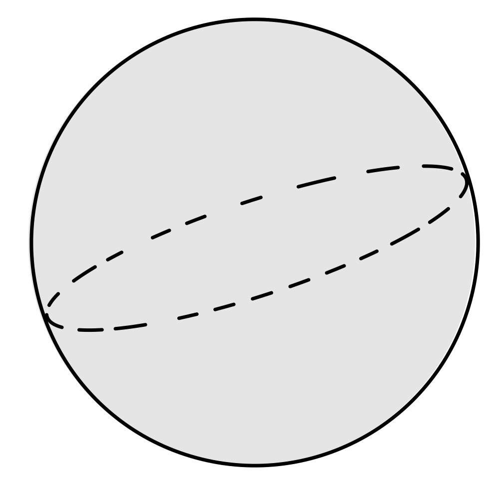
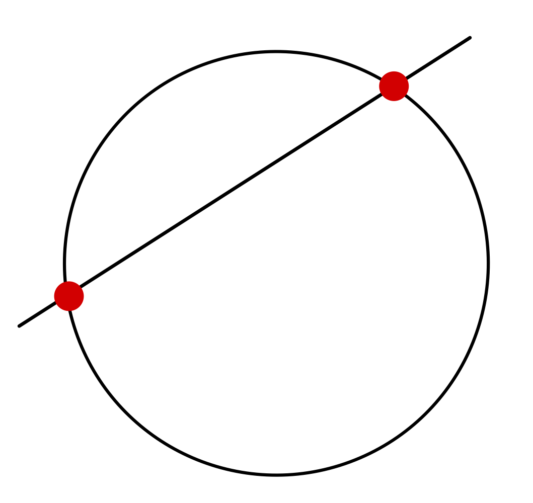
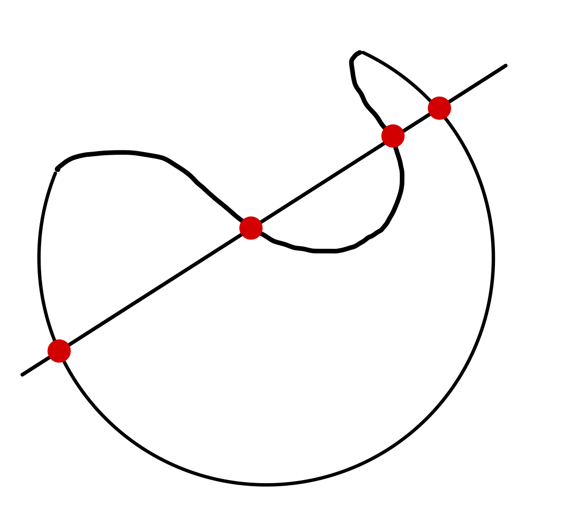
| Closed Surface | Convex | Not Convex |
|---|---|---|
 |  |  |
Definitions
Closed Surface - Divides $3D$ space into $2$ non-connected regions; interior and exterior.
Open Surface - Does not divide $3D$ space into 2 non-connected regions - has a rim which can be represented by closed curve.
Can think of closed surfaces as sum of 2 open surfaces.Convex Surface - A surface which is crossed by a straight line at most twice
Evaluating surface integrals for plane surfaces in x-y plane
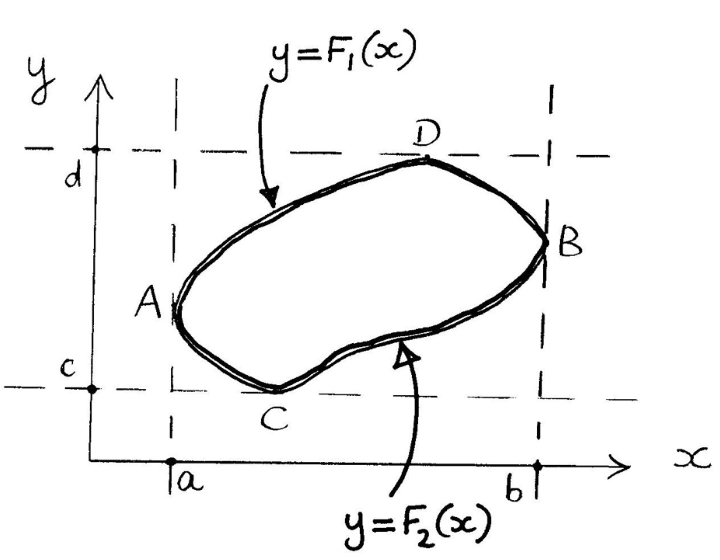
$dS$ infinitesimal area $\implies$ think of as approx. plane.
Vector areal element $dS$ is the vector $\hat{\mathbf{n}}dS$ for $\hat{\mathbf{n}}$ the unit normal vector to $dS$.
For a plane lying in $z = 0$, we can say $dS = dxdy$
For a rectangle, $x = a,b$ and $y = c,d$ circumscribing convex $S$. We let
For $f(x,y)$ a function of position
Equivalently;
Projection of an area onto a plane
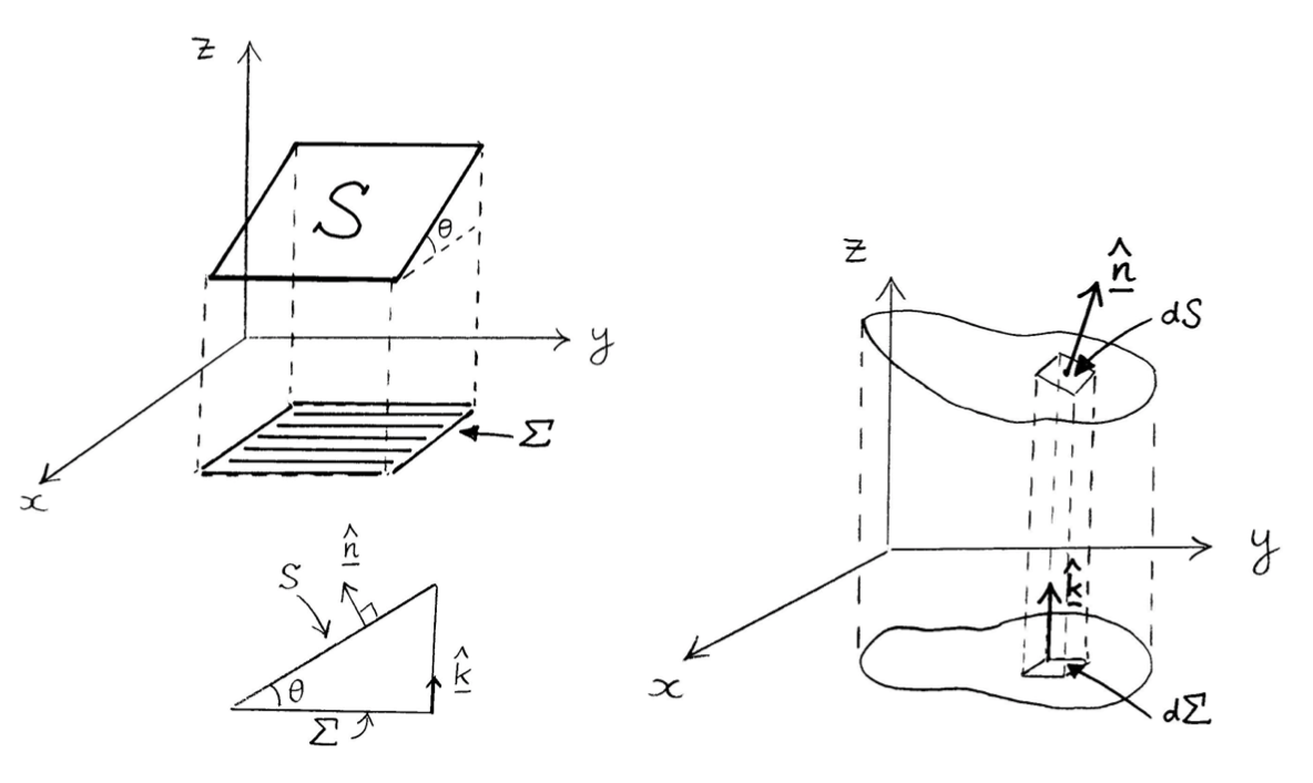
The Projection Theorem
$P$ a point on surface $S$, which at no point is orthogonal to $\mathbf{k}$
For $\Sigma$ a projection of $S$ onto $z= 0$, with $\hat{\mathbf{n}}$ normal to $S$
For $S$ given by $z = \phi(x,y)$
Projecting onto $x =0$ or $y = 0$\
$\Sigma_{x}$, projection onto $x=0$, $\Sigma_{y}$, projection onto $y=0$
Volume Integrals
Definition 1.7.1 - Volume Integral
Considering a volume $\tau$, split into $N$ subregions, ${\delta \tau_{i}}$, with ${P_{i}}$ typical points of ${\delta \tau_{i}}$.
In Cartesian coordinates, the volume element $d \tau = dxdydz$
Results relating line,surface and volume integrals
Green’s Theorem in the plane
$R$ a closed plane region bounded by a simple plane closed convex curve in $x-y$ plane.
$L,M$ continuous functions of $x,y$ with continuous derivatives throughout $R$. Then:
For $C$ the boundary of $R$ described in the counter-clockwise sense.
Vector forms of Green’s Theorem
*(i) $2D$ Stokes Theorem
Let $F = L\mathbf{i} + M\mathbf{j}$ and $d\mathbf{r} = dx\mathbf{i} + dy\mathbf{j}$. Then
Over region $R$ write $dxdy = dS$.
*(ii) Divergence Theorem in $2D$*</span>
Let $\mathbf{F} = M\mathbf{i} - L\mathbf{j}$. Then
So we can rewrite Green’s Theorem as
Green’s Theorem holds for more complicated geometries too, if C not convex we can see it as the composition of 2 or more simple convex closed curves.
Joining $A$, $A’$ form $C_{1}, C_{2}$ enclosing $R_{1},R_{2}$ s.t $R_{1} + R_{2} =R$
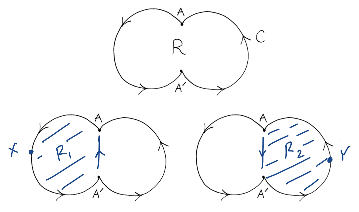
Green’s Theorem in multiply-connected regions
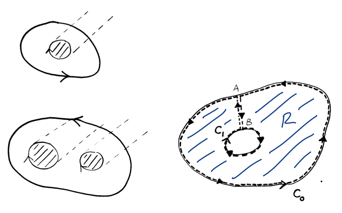
$R$ simply-connected if any closed curve in $R$ can be shrunk to a point without leaving $R$.
For $2D$ any region with a hole in it; not simply connected, we say it is multiply-connected
Green’s theorem still holds in multiply-connected regions.
$C$ interpreted as the entire inner and outer boundary.
For doubly-connected region, describe outer $C_{0}$ anti-clockwise, $C_{1}$ clockwise, and join them via $A$ on $C_{0}$ and $B$ on $C_{1}$
$R$ now a simply connected region bounded by $(C_{0} + AB + C_{1} + BA)$
Where $C = C_{0} + C_{1}$
Flux
If $S$ is a surface then the flux of $A$ across $S$ is defined as
\[\int_{S}\mathbf{A\cdot \hat{n}}dS\]If $S$ a closed surface then by convention draw unit normal $\mathbf{\hat{n}}$ out of $S$.
The divergence theorem
If $\tau$ the volume enclosed by a closed surface $S$ with unit outward normal $\mathbf{\hat{n}}$ and $\mathbf{A}$ is a vector field with continuous derivatives throughout $\tau$, then:
The Divergence theorem in more complicated geometries!
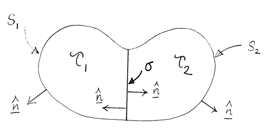
Non-convex surfaces
non-convex surface $S$ can be divided by surfaces(s) $\sigma$ into 2 (or more) parts $S_{1}$ and $S_{2}$ which together with $\sigma$ form convex surfaces $S_{1} + \sigma, S_{2} + \sigma$/
Applying divergence theorem to the convex parts, upon addition yields the same result as before.A region with internal boundaries
Simply-connected regions - e.g space between concentric spheres.
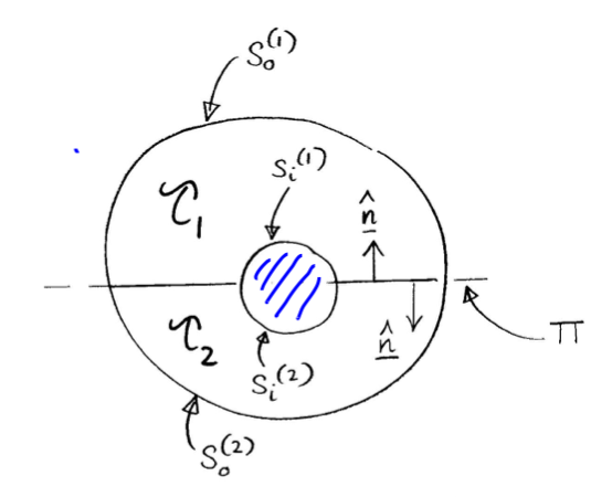
Given interior surface $S_{i}$ and outer surface $S_{o}$. A plane $\Pi$ cutting both $S_{o},S_{i}$, divides $S_{o},S_{i}$ into open $S_{o}^{(1)},S_{o}^{(2)}$ and $S_{i}^{(1)},S_{i}^{(2)}$ respectively.
Apply divergence theorem to $\tau_{1},\tau_{2}$ bounded by closed $S_{o}^{(1)} + S_{i}^{(1)} + \Pi$ and $S_{o}^{(2)} + S_{i}^{(2)} + \Pi$. Upon addition contribution from $\Pi$ cancels. \(\int_{S_{o}+S_{i}}\mathbf{A\cdot \hat{n}}dS = \int_{S}\mathbf{A\cdot \hat{n}}dS = \int_{\tau_{1}}div \mathbf{A}d\tau + \int_{\tau_{2}}div \mathbf{A}d\tau = \int_{\tau}div \mathbf{A}d\tau\)Multiply-connected regions
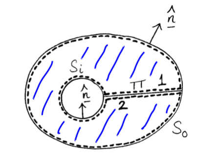
e.g. region between 2 cyclinders.
Given interior surface $S_{i}$ and outer surface $S_{o}$, linked by plane $\Pi$.
Consider the closed surface, enclosing simply connected region $\tau$$S_{i} +$ side 1 of $\Pi+ S_{o} +$ side 2 of $\Pi$ Applying divergence theorem to $\tau$. Once again gives \(\int_{S_{0}+S_{i}}\mathbf{A\cdot\hat{n}}dS = \int_{\tau}div\mathbf{A}d\tau\)
Green’s identity in 3D
For $\phi$ and $\psi$ 2 scalar fields with continuous derivatives. We consider $\mathbf{A} = \phi \nabla \psi$, for which we have
Green’s first identity
Green’s Second identity
Green’s identities in 2D
Divergence theorem in 2D: $\int_{F}div \mathbf{F}dxdy = \oint_{C}\mathbf{F\cdot\hat{n}}ds$
Giving the following Green’s identities:
and
$\int_{R}\phi\nabla^{2}\psi\ dxdy = \oint_{C}\phi \frac{\partial \psi}{\partial n}ds - \int_{R}(\nabla\psi)\cdot(\nabla\phi)dxdy$ - Looks like Integration by parts
Gauss’ Flux Theorem
Let $S$ a closed surface with outward unit normal $\mathbf{\hat{n}}$ and let $O$ the origin of the coordinate system.
$\mathbf{A} = \frac{\mathbf{r}}{r^{3}}$ Then:
Stokes Theorem
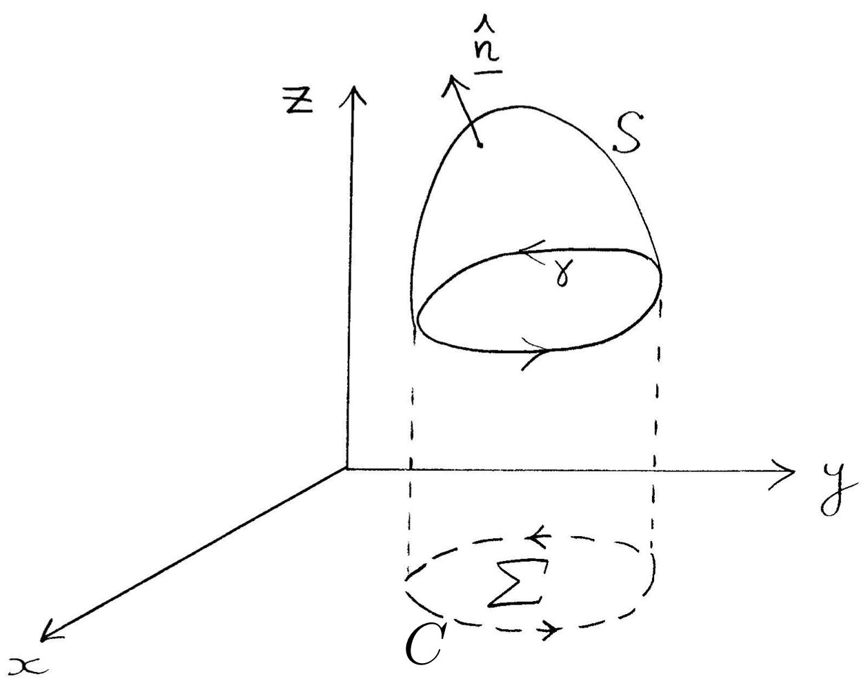
Suppose $S$ is open surface with simple closed curve $\gamma$ forming its boundary.
$A$ a vector field with continuous partial derivatives, Then:
This holds for any open surface with $\gamma$ as a boundary.
Theorem
For $\mathbf{A}$ continuously differentiable and simply connected region:
Curvilinear Coordinates
Intro + Definition
Consider generally cartesian coordinates: $(x_1,x_2,x_3)$ with each expressible as single-valued differentiable functions of the new coorinates $(u_1,u_2,u_3)$
Or more succinctly
We say $J(x_u)$ the Jacobian matrix for the $(x_1,x_2,x_3)$ system.
We say $(u_1,u_2,u_3)$ define a curvilinear coordinate system.
With each $u_i =$ constant, defining a family of surfaces, with a member of each family passing through each $P(x,y,z)$
Let $(\hat{\mathbf{a}}{1},\hat{\mathbf{a}}{2},\hat{\mathbf{a}}{3})$ unit vectors at $P$ in the direction normal to $u{i} = u_{i}(P)$, s.t $u_{i}$ increasing in the direction $\hat{\mathbf{a}}_{i}$
if we have that $\mathbf{(\hat{a_1},\hat{a_2},\hat{a_3})}$ mutually orthogonal $\implies$ orthogonal curvilinear coordinate system.
For which we define $h_{i} = \lvert \partial \mathbf{r}/ \partial u_{i} \rvert$. We call these the length scales
Path element
$\mathbf{r} = \mathbf{r}(u_1,u_2,u_3)$ path element $d\mathbf{r}$ given by
For an orthogonal system
Volume Element
Surface element
For $u_1$ constant. \(dS = h_2h_3du_2du_3\) similarly for $u_2,u_3$
Properties of various orthogonal coordinates
Cartesisan coordinates $(x,y,z)$
$$ \begin{aligned} d\tau &= dxdydz & d\mathbf{r} &= dx\mathbf{\hat{i}} + dy\mathbf{\hat{j}} + dz\\ \mathbf{\hat{k}} (ds)^{2} &= (d\mathbf{r})\cdot(d\mathbf{r}) = (dx)^{2} + (dy)^{2} + (dz)^{2} \end{aligned} $$ We have $h_{1} = h_{2} = h_{3}$
Cylindrical polar coordinates $(r,\phi,z)$
\[x = r\cos \theta \quad y = r\sin \phi \quad z = z\] \[\begin{aligned} \frac{\partial \mathbf{r}}{\partial r} &= (\frac{\partial x}{\partial r})\mathbf{\hat{i}} + (\frac{\partial y}{\partial r})\mathbf{\hat{j}} + (\frac{\partial z}{\partial r})\mathbf{\hat{k}} \hspace{1.5pt} = (\cos\phi)\mathbf{\hat{i}} + (\sin\phi)\mathbf{\hat{j}}\\ \frac{\partial \mathbf{r}}{\partial \phi} &= (\frac{\partial x}{\partial \phi})\mathbf{\hat{i}} + (\frac{\partial y}{\partial \phi})\mathbf{\hat{j}} + (\frac{\partial z}{\partial \phi})\mathbf{\hat{k}} = -(r\sin\phi)\mathbf{\hat{i}} + (r\cos\phi)\mathbf{\hat{j}}\\ \frac{\partial \mathbf{r}}{\partial z} &= \mathbf{\hat{k}} \end{aligned}\] \[\begin{aligned} (\frac{\partial \mathbf{r}}{\partial r})\cdot(\frac{\partial \mathbf{r}}{\partial \phi}) &= 0\\ (\frac{\partial \mathbf{r}}{\partial r})\cdot(\frac{\partial z}{\partial \phi}) &= 0\\ (\frac{\partial \mathbf{r}}{\partial \phi})\cdot(\frac{\partial \mathbf{r}}{\partial z}) &= 0 \end{aligned}\] \[\begin{aligned} h_{1} &= \lvert \frac{\partial \mathbf{r}}{\partial r} \rvert = 1\\ h_{2} &= \lvert \frac{\partial \mathbf{r}}{\partial \phi} \rvert = r\\ h_{3} &= \lvert \frac{\partial \mathbf{r}}{\partial z} \rvert = 1 \end{aligned}\]
Related to cartesian byYielding length and volume elements:
\[\begin{aligned} (ds)^2 &= (dr)^2+r^2(d)^2+(dz)^2 \end{aligned}\] \[\begin{aligned} d= rdrddz \end{aligned}\]Spherical polar coordinates $(r,\theta,\phi)$
\[x = r\sin\theta\cos\phi \quad y = r\sin\theta\sin\phi \quad z = r\cos\theta\] \[\theta \in [0,\pi],\ \phi \in [0,2\pi]\] \[\begin{aligned} \frac{\partial \mathbf{r}}{\partial r} &= (\sin\theta\cos\phi)\mathbf{\hat{i}} + (\sin\theta\sin\phi)\mathbf{\hat{j}} + (\cos\theta)\mathbf{\hat{k}} \\ \frac{\partial \mathbf{r}}{\partial \theta} &= (r\cos\theta\cos\phi)\mathbf{\hat{i}} + (r\cos\theta\sin\phi)\mathbf{\hat{j}} + (-r\sin\theta)\mathbf{\hat{k}} \\ \frac{\partial \mathbf{r}}{\partial \phi} &= (-r\sin\theta\sin\phi)\mathbf{\hat{i}} + (r\sin\theta\cos\phi)\mathbf{\hat{j}} + (0)\mathbf{\hat{k}} \end{aligned}\] \[\begin{aligned} (\frac{\partial \mathbf{r}}{\partial r})\cdot(\frac{\partial \mathbf{r}}{\partial \theta}) &= 0\\ (\frac{\partial \mathbf{r}}{\partial r})\cdot(\frac{\partial \mathbf{r}}{\partial \phi}) &= 0\\ (\frac{\partial \mathbf{r}}{\partial \phi})\cdot(\frac{\partial \mathbf{r}}{\partial \theta}) &= 0 \end{aligned}\] \[\begin{aligned} h_{1} &= \lvert \frac{\partial \mathbf{r}}{\partial r} \rvert = 1\\ h_{2} &= \lvert \frac{\partial \mathbf{r}}{\partial \theta} \rvert = r\\ h_{3} &= \lvert \frac{\partial \mathbf{r}}{\partial \phi} \rvert = r\sin\theta \end{aligned}\]
Related to cartesian by:Volume element:
\[d\tau = r^{2}\sin\theta drd\theta d\phi\]
Gradient in orthogonal curvilinear coordinates
Let $\nabla\Phi = \lambda_{1}\mathbf{\hat{e}}{1} + \lambda{2}\mathbf{\hat{e}}{2} + \lambda{3}\mathbf{\hat{e}}_{3}$
In a general coordinate system for $\lambda_{i}$s to be found.
\[d\mathbf{r} = h_{1}du_{1}\hat{e}_{1} + h_{2}du_{2}\hat{e}_{2} + h_{3}du_{3}\hat{e}_{3}\] \[\begin{aligned} d\mathbf{\Phi} &= (\frac{\partial \phi}{\partial u_{1}})du_{1} + (\frac{\partial \phi}{\partial u_{2}})du_{2}+ (\frac{\partial \phi}{\partial u_{3}})du_{3}\\ &= (\frac{\partial \phi}{\partial x})dx + (\frac{\partial \phi}{\partial y})dy+ (\frac{\partial \phi}{\partial z})dz\\ &= (\nabla\Phi)\cdot d\mathbf{r} = \lambda_{1}h_{1}du_{1} + \lambda_{2}h_{2}du_{2} + \lambda_{3}h_{3}du_{3} \end{aligned}\] \[h_{i}\lambda_{i} = \frac{\partial \Phi}{\partial u_{i}}\] \[\implies \nabla \Phi = \frac{\hat{\mathbf{e}}_{1}}{h_{1}}\frac{\partial \Phi}{\partial u_{1}} + \frac{\hat{\mathbf{e}}_{2}}{h_{2}}\frac{\partial \Phi}{\partial u_{2}} + \frac{\hat{\mathbf{e}}_{3}}{h_{3}}\frac{\partial \Phi}{\partial u_{3}}\]Cylindrical polars $(r,\phi,z)$
\[\implies \begin{aligned} \nabla = \hat{r}\frac{\partial}{\partial r} + \frac{\hat{\phi}}{r}\frac{\partial}{\partial \phi} + \hat{z}\frac{\partial}{\partial z} \end{aligned}\]
We have: $\begin{aligned} h_{1} &= 1
h_{2} &= r
h_{3} &= 1 \end{aligned}$Spherical polars $(r,\theta,\phi)$
\[\begin{aligned} h_1 &= 1\\ h_2 &= r\\ h_3 &= r \end{aligned}\] \[\implies \begin{aligned} \nabla = \hat{r}\frac{\partial}{\partial r} + \frac{\hat{\theta}}{r}\frac{\partial}{\partial \theta} + \frac{\hat{\phi}}{r\sin\theta}\frac{\partial}{\partial \phi} \end{aligned}\]
We have:
Expressions for unit vectors
Alternatively, unit vectors orthogonal $\implies$ if we know 2 already then
Divergence in orthogonal curvilinear coordinates
Suppose we have vector field
So we have divergence in other coordinate systems as follows:
Curl in orthogonal curvilinear coordinates
- Cylindrical polars
$$curl \mathbf{A} = \frac{1}{r} \begin{vmatrix} \mathbf{\hat{r}} & r\hat{\phi} & \mathbf{\hat{k}}\\ \partial/\partial r & \partial/\partial \phi & \partial/\partial z\\ A_1 & A2 & A_3 \end{vmatrix}$$ - Spherical polars
$$curl \mathbf{A} = \frac{1}{r^{2}\sin\theta} \begin{vmatrix} \mathbf{\hat{r}} & r\hat{\phi} & r\sin\theta\hat{\phi} \\ \partial/\partial r & \partial/\partial \phi & \partial/\partial z\\ A_1 & rA2 & r\sin\theta A_3 \end{vmatrix}$$
The Laplacian in orthogonal curvilinear coordinates
From the above grad and div;
- Cylindrical polars $(r,\phi,z)$
$$\begin{aligned} \nabla^{2}\Phi &= \frac{1}{r}\left \{ \frac{\partial}{\partial r}\left ( r\frac{\partial \Phi}{\partial r} \right ) + \frac{\partial}{\partial \phi}\left ( \frac{1}{r}\frac{\partial \Phi}{\partial \phi} \right ) + \frac{\partial}{\partial z}\left ( r\frac{\partial \Phi}{\partial z} \right ) \right \} \\ &= \frac{\partial^{2}\Phi}{\partial r^{2}} + \frac{1}{r}\frac{\partial \Phi}{\partial r} + \frac{1}{r^{2}}\frac{\partial^{2}\Phi}{\partial \phi^{2}} + \frac{\partial^{2}\Phi}{\partial z^{2}} \end{aligned}$$ - Spherical polars $(r,\theta,\phi)$
$$\begin{aligned} \nabla^{2}\Phi &= \frac{1}{r^{2}\sin\theta}\left \{ \frac{\partial}{\partial r}\left ( r^{2}\sin\theta\frac{\partial \Phi}{\partial r} \right ) + \frac{\partial}{\partial \theta}\left ( \sin\theta\frac{\partial \Phi}{\partial \theta} \right ) + \frac{\partial}{\partial \phi}\left ( \frac{1}{\sin\theta}\frac{\partial \Phi}{\partial \phi} \right ) \right \} \\ &= \frac{\partial^{2}\Phi}{\partial r^{2}} + \frac{2}{r}\frac{\partial \Phi}{\partial r} + \frac{\cot\theta}{r^{2}}\frac{\partial\Phi}{\partial \theta} + \frac{1}{r^{2}}\frac{\partial^{2}\Phi}{\partial \theta^{2}} + \frac{1}{r^{2}\sin^{2}\theta}\frac{\partial^{2}\Phi}{\partial \phi^{2}} \end{aligned}$$
Changes of variables in surface integration
Suppose we have surface $S$, parametrized by quantities $u_1,u_2$. We can write:
Consider surface to be comprised of arbitrarily small parallelograms, its sides given by keeping either $u_1$ or $u_2$
Vector Jacobian given by $\mathbf{J} = \frac{d\mathbf{r}}{du_1}\times\frac{d\mathbf{r}}{du_2}$.
Useful in substitution of surface integrals:
$F(u_1,u_2) = f(x(u_1,u_2),y(u_1,u_2),z(u_1,u_2))$
For S a region $R$ in the $x-y$ plane we can write:
For a surface described by $z = f(x,y)$. We have $x = u_1, y = u_2$ and $\mathbf{r} = (x,y,f(x,y))$
We have:
\[\begin{aligned} \frac{\partial \mathbf{r}}{\partial u_1} &= \frac{\partial \mathbf{r}}{\partial x} \hspace{-2pt} &= \mathbf{\hat{i}} + \frac{\partial f}{\partial x}\mathbf{\hat{k}}\\ \frac{\partial \mathbf{r}}{\partial u_2} &= \frac{\partial \mathbf{r}}{\partial y} \hspace{-2pt} &= \mathbf{\hat{j}} + \frac{\partial f}{\partial y}\mathbf{\hat{k}}\\ \end{aligned}\]So we have area of surface given by
for $\Sigma$ the projection of $S$ onto the $x-y$ plane.
Term II
Introduction
ODEs and initial value problems
Definition 1.2. Ordinary differential equation
Consider $d \in \mathbb{N}$ an open set $D \subset \mathbb{R}\times \mathbb{R}^{d}$ and function $f:D \to \mathbb{R}^{d}$ Call
\[\dot{x} = f(t,x)\]a d-dimensional (first-order) ordinary differential equation
Differentiable function $\lambda:I \to \mathbb{R}^{d}$ on interval $I \subset \mathbb{R}$ a solution to a differential equation if $(t,\lambda(t)) \in D$ and
\[\dot{\lambda}(t) = f(t,\lambda(t))\quad \forall t \in I\]Say ODE autonomous if of form
\[\dot{x} = f(x)\]for $f:D\to\mathbb{R}^{d}, D\subset \mathbb{R}^{d}$
Proposition 1.3.
$D \subset \mathbb{R}^{d}$ open. $f:D \to \mathbb{R}^{d}$ with autonomous ODE \(\dot{x} = f(x)\) $\implies \exists$ constant solution $\lambda:\mathbb{R}\to\mathbb{R}^{d}$ with $a \in \mathbb{R}^{d}$ at $\lambda(t) = a \iff f(a) =0 \forall t$
Definition 1.4. Initial value problem
$d \in \mathbb{N}$ open $D \subset \mathbb{R}\times\mathbb{R}^d,\ f:D \to \mathbb{R}^d$.
Call the following pair a initial value problem
Solutions s.t $\lambda:I \to \mathbb{R}^d$ with $t_0$ in interior of $I$ and $\lambda(t_0) = x_0$
Visualisations
Solution portrait
$f:D \subset \mathbb{R}\times\mathbb{R}^d \to \mathbb{R}^d$ with $\dot{x} = f(t,x)$
Graph of solutions given by
Solution Curve
\[G(\lambda) = \left\{(t,\lambda(t)): t \in I\right\} \subset \mathbb{R}\times \mathbb{R}^d\]derivative of curve at point $t_0 \in I$ is
\[\frac{d}{dt}(t,\lambda(t))\vert_{t = t_0} = (t,\dot{\lambda}(t_0)) = (1, f(t_0,\lambda(t_0))\]Vector field a map $(t,x) \mapsto (1,f(t,x))$, defined on $D$
Solution Curves are tangential to vector field.
Solution portrait given by visualisations of several solution curves in both
Phase Portraits
Autonomous differential equations not dependent on time. Visualisations in phase-space alone suffice.
Proposition 1.9.(Translation invariance)
$\lambda: I \to \mathbb{R}^{d}$ a solution to $\dot{x} = f(x)$
$\implies \forall \tau \in \mathbb{R}, \mu: \tilde{I}\to \mathbb{R}^{d}$
where $\tilde{I} = {t\in \mathbb{R}: t+ \tau \in I}$
$\mu(t) = \lambda(t+ \tau),\ \forall t \in \tilde{I}$ also a solution to this differential equation.
Existence & Uniqueness
Picard iterates
Proposition 2.1. - (Reformation as integral equation)
Consider initial value problem $\dot{x} = f(t,x),\quad x(t_0) = x_0$
for $f: D\subset \mathbb{R}\times\mathbb{R}^{d} \to \mathbb{R}^{d}$ continuous and $(t_0,x_0) \in D$
$\lambda: I \to \mathbb{R}^{d}$ a function on interval $I$ s.t $t_0 \in I$ and ${(t,\lambda(t)): t \in I} \subset D$
Following are equivalent:
$\lambda$ solves initial value problem
$\dot{\lambda}(t) = f(t,\lambda(t)),\ \forall t \in I$
$\lambda(t_0) = x_0$$\lambda$ continuous and \(\lambda(t) = x_0 + \int_{t_0}^{t}f(s,\lambda(s))ds\ \forall t \in I\)
Higher dimensional derivative
for $g:\mathbb{R}\to\mathbb{R}^{d}$
Definition 3. (Picard iterates)
Consider initial value problem; $\dot{x} = f(t,x)\quad x(t_0) = x_0$ and chosen interval $J$ s.t $t_0 \in J$
Define initial function:
and inductively the Picard iterates:
\[\lambda_{n+1}(t) := x_0 + \int_{t_0}^{t}f(s,\lambda_n(s))ds \quad \forall t\in J\ \forall n \in \mathbb{N}_{0}\]If $(\lambda_n)$ uniformly convergent sequence with limit $\lambda_{\infty}$ obtain:
\[\lambda_{\infty}(t) = x_0 + \int_{t_0}^{t}f(s,\lambda_{\infty}(s))ds\ \forall t \in J\]$\implies \lambda_{\infty}$ a solution to integral equation $\implies$ solves initial value problem
Lipschitz Continuity
Definition
Space of continuous functions on compact interval J $:= C^{0}(J,\mathbb{R}^{d})$
This a complete normed vector space under supremum norm. (Banach Space)
Definition 4. (Normed Vector Space)
Norm on a vector space $V$ over $\mathbb{R}$ a map $\lvert \lvert \cdot\rvert\rvert:V \to \mathbb{R}^{+}_{0}$ s.t
$\lvert \lvert x\rvert\rvert = 0 \iff x = 0$
$\lvert \lvert ax\rvert\rvert = \lvert a\rvert\cdot\lvert \lvert x\rvert\rvert,\ \forall a \in \mathbb{R},x \in V$
$\lvert \lvert x+y\rvert\rvert\leq \lvert \lvert x\rvert\rvert+\lvert \lvert y\rvert\rvert$
Normed vector space $V$ complete if every cauchy sequence converges in $V$
Call a complete normed vector space a Banach Space
Definition 5. (Continuous + Lipschitz continuous functions)
$X \subset$ normed vector space $(V,\lvert \lvert \cdot\rvert\rvert_{V})$
$Y \subset$ normed vector space $(W,\lvert \lvert \cdot\rvert\rvert_{W})$
We say a function $f:X \to Y$
Continuous if
\[\forall x \in X, \epsilon > 0, \exists \delta > 0, \lvert \lvert x-\bar{x}\rvert\rvert_{V} < d \implies \lvert \lvert f(x)-f(\bar{x})\rvert\rvert_{W} < \epsilon\]Lipschitz Continuous if
\[\exists K > 0, \lvert \lvert f(x)-f(\bar{x})\rvert\rvert_{W} \leq K\lvert \lvert x-\bar{x}\rvert\rvert_{V}\ \forall x,\bar{x} \in X\]Call $K$ a Lipschitz Constant
Lipschitz continuous $\implies$ Continuous
Lipschitz Continuity and MVT
Theorem 1. (Mean Value Theorem)
$I$ compact interval, $f$ continuously differentiable
$\forall x,y \in I,\ \exists \xi \in (x,y)$ s.t
$f(x)- f(y) = f’(\xi)(x-y)$
$\implies f’$ bounded $\implies$ $f$ Lipschitz continuous
Lipschitz Continuity and Mean Value Inequality
Definition 6. (Operator norm of a matrix)
For given matrix $A \in M_n(\mathbb{R})$ Operator norm:
\[\lvert \lvert A\rvert\rvert = \sup_{x\in\mathbb{R}^{n}\backslash\{0\}}\frac{\lvert \lvert Ax\rvert\rvert}{\lvert \lvert x\rvert\rvert} = \sup_{x\in\mathbb{R}^{n}\backslash\{0\}}\left|\left|A\frac{x}{\lvert \lvert x\rvert\rvert}\right|\right| = \sup_{x\in \mathbb{R}^{n},\lvert \lvert x\rvert\rvert = 1}\lvert \lvert Ax\rvert\rvert\]Theorem 2. (Mean Value Inequality)
Consider open set $D \subset \mathbb{R}^{n}$ with $f:D \to \mathbb{R}^{m}$ continuously differentiable
$\forall x,y \in D$ with $[x,y] \subset D$
$\forall x,y \in \mathbb{R}^{n}$, closed line segment connecting $x$ and $y$ given by
\[[x,y] = \{\alpha x + (1-\alpha)y \in \mathbb{R}^{n} : \alpha \in [0,1]\}\]Lemma 2.9. (Triangle-like inequality for integrals)
$I \subset R$ an interval
$f:I \to \mathbb{R}^{m}$ continuous function
Corollary 2.10. - (Lipschitz continuous and mean value inequality)
$U \subset \mathbb{R}^{n}$ open. $f:U \to \mathbb{R}^{m}$ continuously differentiable
Given compact and convex set $C\subset U$. Restriction is Lipschitz continuous
Convex $C$ means $\forall x,y, \in C$ closed line segment lies in $C$ i.e. $[x,y] \subset C$
Picard-Lindelöf Theorem
Theorem 3. (Picard-Lindelöf theorem - global version)
Consider ODE $\dot{x} = f(t,x)$
$f:\mathbb{R}\times\mathbb{R}^d \to \mathbb{R}^d$ continuous, satisfying global Lipschitz condition of the form
Take $h = \frac{1}{2K} \implies$ every intial value problem $x(t_0) = x_0$ admits a unique solution
\[\lambda:[t_0 - h, t_0 + h] \to \mathbb{R}^d\]Definition 7.
Globally Lipschitz continuous
if $\exists K > 0$ s.t $\lvert \lvert f(t,x) - f(t,y) \rvert\rvert \leq K \lvert \lvert x-y \rvert\rvert \quad \forall (t,x),(t,y) \in D$Locally Lipschitz continuous
\[\lvert \lvert f(t,x) - f(t,y) \rvert\rvert \leq K \lvert \lvert x - y \rvert\rvert \quad \forall (t,x),(t,y) \in U\]
if $\forall (t_0,x_0) \in D$ and $\exists$ neighbourhood $U\subset D$ of $(t_0,x_0)$ and $\exists L > 0$ s.t
Theorem 4. (Picard-Lindelöf theorem - local version)
$D \subset \mathbb{R}\times \mathbb{R}^{d}$ open
Consider function $f: D \to \mathbb{R}^d$ continuous and locally Lipschitz continuous.
For fixed $(t_0,x_0) \in D$, we have intial value problem. Following 2 hold
Qualitative version
\[\exists h = h(t_0,x_0) \text{ s.t. there is exactly one solution on } [t_0-h,t_0 + h]\]
Initial value problem has locally a uniquely determined solutionQuantitative version
\[\lvert \lvert f(t,x) - f(t,y) \rvert\rvert \leq K \lvert \lvert x - y \rvert\rvert \quad \forall (t,x),(t,y) \in U\]
For some $\tau,\delta$ take set $W^{\tau,\delta}(t_0,x_0) := [t_0-\tau,t_0+\tau] \times \overline{B_{\delta}(x_0)}$. For $\overline{B_{\delta}(x_0)} := { x\in \mathbb{R}^d:\lvert \lvert x- x_0 \rvert\rvert \leq \delta }$ - Closed $\delta-$neighbourhood of $x_0$.
Assume $W^{\tau,\delta}(t_0,x_0) \subset D$, suppose $\exists K,M > 0$ s.tand
\[\lvert \lvert f(t,x) \rvert\rvert \leq M \quad \forall (t,x) \in W^{\tau,\delta}(t_0,x_0)\]$\implies$ there is exactly one solution on $[t_0-h,t_0+h]$ with $h(t_0,x_0) := \min{\tau,\frac{1}{2K},\frac{\delta}{M}}$
Proposition 2.14. - (Continuously differentiable & Lipschitz Continuity)
$D\subset \mathbb{R}\times \mathbb{R}^d$ open. Continuously differentiable function $f:D\to \mathbb{R}^d$
Lemma 2.15. - (Solutions cannot cross)
Let $D \subset \mathbb{R}\times \mathbb{R}^d$ open. $f:D \to \mathbb{R}^d$ continuous and locally Lipschitz continuous w.r.t $x$
Given 2 solutions of $\dot{x} = f(t,x)$; $\lambda: I \to \mathbb{R}^d, \mu: J \to \mathbb{R}^d$
Either $\lambda(t) = \mu(t) \quad \forall t \in I \cap J$ or $\lambda(t) \neq \mu(t) \quad \forall t \in I \cap J$
Maximal Solutions
Definition 8. - (Maximal existence interval)
Consider initial value problem $\dot{x} = f(t,x),\ x(t_0) = x_0$ Define
$I_{+}(t_0,x_0) := \sup{ t_{+} \geq t_0 : \text{there exists solution on } [t_0,t_{+}] }$
$I_{-}(t_0,x_0) := \sup{ t_{-} \leq t_0 : \text{there exists solution on } [t_{-},t_0] }$
Maximal existence interval:
\[I_{max}(t_0,x_0) := \left( I_{-}(t_0,x_0), I_{+}(t_0,x_0) \right)\]Theorem 5. (Existence of maximal solution + boundary behaviour)
There exists maximal solution $\lambda_{max}:I_{max}(t_0,x_0) \to \mathbb{R}^d$ to initial value problem. Having properties:
$I_{+}(t_0,x_0)$ finite
\[\sup_{t \in (t_0,I_{+}(t_0,x_0))} \lvert \lvert \lambda_{max}(t) \rvert\rvert = \infty\]
Either - maximal solution unbounded for $t\geq t_0$Or boundary: $\partial D$ of $D$ non-empty and we have
\[\lim_{t \nearrow I_{+}(t_0,x_0)} dist\left( (t,\lambda_{max}(t)),\partial D\right) = 0\]$I_{-}(t_0,x_0)$ finite
\[\sup_{t \in (I_{-}(t_0,x_0),t_0)} \lvert \lvert \lambda_{max}(t) \rvert\rvert = \infty\]
Either - maximal solution unbounded for $t \leq t_0$Or boundary: $\partial D$ of $D$ non-empty and we have
\[\lim_{t \searrow I_{-}(t_0,x_0)} dist\left( (t,\lambda_{max}(t)),\partial D\right) = 0\]
Dist function
$A \subset \mathbb{R}^{n},\ dist(\cdot,A):\mathbb{R}^n \to \mathbb{R}_{0}^{+}$
\[dist(y,A) := \inf\{\lvert \lvert y-a\rvert\rvert: a \in A\} \quad \forall y \in \mathbb{R}^n\]General solutions and flows
General solutions
Definition 9. (General solution to non-autonomous differential equation)
Consider $\dot{x} = f(t,x)$. We define
\[\Omega := \{ (t,t_0,x_0) \in \mathbb{R}^{1+1+d}: (t_0,x_0) \in D \text{ and } t\in I_{max}(t_0,x_0) \}\]We say $\lambda:\Omega \to \mathbb{R}^{d}$ with $\lambda(t,t_0,x_0) := \lambda_{max}(t,t_0,x_0)$ a general solution of $\dot{x} = f(t,x)$
Solution identity:
\[\frac{\partial \lambda}{\partial t}(t,t_0,x_0) = f(t,\lambda(t,t_0,x_0)) \quad \forall (t,t_0,x_0) \in \Omega\]Proposition 2.21. - (Properties of general solutions)
Consider $\dot{x} =f(t,x)$, $(t_0,x_0) \in D$ $\implies \forall s \in I_{max}(t_0,x_0)$ we have
$I_{max}(s,\lambda(s,t_0,x_0)) = I_{max}(t_0,x_0)$
$\lambda(t_0,t_0,x_0) = x_0$ (Initial value property)
$\lambda(t,s,\lambda(s,t_0,x_0)) = \lambda(t,t_0,x_0) \forall t \in I_{max}(t_0,x_0)$ (Cocycle property)
Flows
Definition 10. (Flow of an autonomous differential equation)
Consider $\dot{x} = f(x)$
Define for any initial value $x_0 \in D$
$(t,x_0) \mapsto \phi(t,0,x_0)$ called flow of autonomous differential equation
Solution identity:
\[\frac{\partial \varphi}{\partial t}(t,x_0) = f(\varphi(t,x_0)) \quad \forall x_0 \in D, t \in J_{max}(0)\]Proposition 2.24 - (Properties of the flow)
Let $\varphi$ be flow of autonomous differential equation. $\implies \forall x \in D$ we have
$J_{max}(\varphi(t,x)) = J_{max}(x) - t \quad \forall t \in J_{max}(x)$
$\varphi(0,x) = x$ (Initial value property)
$\varphi(t,\varphi(s,x)) = \varphi(t +s ,x) \quad \forall t,s$ with $s,t+s \in J_{max}(x)$ (Group property)
$\varphi(-t,\varphi(t,x)) = x \quad \forall t \in J_{max}(x)$
Definition 11. (Orbits (or trajectories))
$\varphi$ flow of autonomous differential equations $\forall x \in D$, we have the Orbit through $x$
\[O(x) := \{ \varphi(t,x) \in D: t \in J_{max}(x) \}\]With the positive/negative half orbits:
$O^{+}(x) := { \varphi(t,x) \in D: t \in J_{max}(x) \cap \mathbb{R}^{+}_{0}}$
$O^{-}(x) := { \varphi(t,x) \in D: t \in J_{max}(x) \cap \mathbb{R}^{-}_{0}}$
Types of orbits
$O(x)$ singleton $\implies f(x) = 0$ and $J_{max}(x) = \mathbb{R}$
Call $x$ the equilibrium$O(x)$ closed curve $\exists t> 0$ s.t $\varphi(t,x) = x$ but $f(x) \neq 0$ $\implies$ $J_{max}(x) = \mathbb{R}$, call $x$ periods with $O(x)$ periodic orbit
$O(x)$ not closed curve. function $t \mapsto \varphi(t,x)$ injective on $J_{max}(x)$
Proposition 2.27. - (Orbits of one-dimensional differential equation)
Consider $\dot{x} = f(x)$ where $d = 1$
$\implies$ all solutions monotone, $\not\exists$ periodic orbits
$\implies$ trajectory either an equilibrium or non-closed curve
Linear Systems
Matrix exponential function
Consider linear differential equation
\(\dot{x} = Ax \quad A \in \mathbb{R}^{d\times d}\) We have $\lvert \lvert Ax - Ay\rvert\rvert \leq \lvert \lvert A\rvert\rvert \lvert \lvert x-y\rvert\rvert$
$\implies$ globally Lipschitz continuous with constant $\lvert \lvert A \rvert\rvert$\
Solution to every intial value problem exists and are unique.
$\implies$ generates globally defined flow $\varphi: \mathbb{R}\times \mathbb{R}^d \to \mathbb{R}^d$
Picard iterates for local solutions
$\lambda_{0}(t) := x_0 \forall t \in J$
$\lambda_{n+1} = P(\lambda_n)(t) = x_{0} + \int_{0}^{t}A\lambda_n(s)ds \implies \lambda_n = \sum_{k=0}^{n} \frac{t^k A^k}{k!}x_0$
$\implies \lambda_{\infty}(t) = \varphi(t,x_0) e^{At}x_0$
We have the series converge whenever $\lvert t \rvert \leq h$ for some $h >0$
Definition 12. (Matrix exponential function)
\[t \mapsto e^{At} \qquad e^{At} = \sum_{k = 0}^{\infty}\frac{t^k A^k}{k!}\]Lemma 3.1.
\[\lvert \lvert BC \rvert\rvert \leq \lvert \lvert B \rvert\rvert \lvert \lvert C \rvert\rvert\]Proposition 3.2. - (Existence of matrix exponential)
Matrix $B \in \mathbb{R}^{d\times d}$
\(e^{B} := \sum_{k=0}^{\infty}\frac{1}{k!}B^{k} \in \mathbb{R}^{d\times d}\) exists
Theorem 6. (Flow of an autonomous linear differential equation)
Consider $\dot{x} = Ax, \quad A \in \mathbb{R}^{d\times d}$
Flow $\varphi: \mathbb{R}\times \mathbb{R}^d \to \mathbb{R}^d$ given by
Proposition 3.4. - (Properties of matrix exponential)
$C = T^{-1}BT \implies e^{C} = T^{-1}e^{B}T$
$e^{-B} = (e^{B})^{-1}$
$BC = CB \implies e^{B+C} = e^{B}e^{C}$
$B = diag(B_{1},\dots,B_p) \implies e^B = diag(e^{B_1},\dots,e^{B_p})$
Planar linear systems
Consider $\dot{x} = Ax, A \in \mathbb{R}^{2\times 2}$
Transform $A$ in Jordan normal form $\implies J = T^{-1}AT$, $T$ invertible
$\implies e^{AT} = Te^{Jt}T^{-1}$
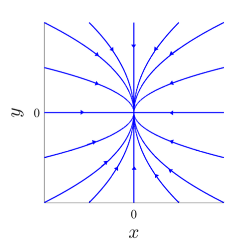
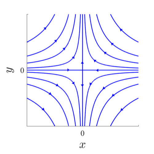
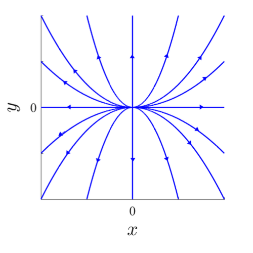
C1. $A$ has $2$ distinct real eigenvalues, $a,b \in \mathbb{R}$ \(J = \begin{pmatrix}a & 0\\ 0 & b\end{pmatrix}\)
C2. $A$ has double real eigenvalues $a \in \mathbb{R}$, with $2$ linearly independent eigenvectors \(J = \begin{pmatrix}a & 0\\ 0 & a\end{pmatrix}\)
C3. $A$ double real eigenvalues with $1$ eigenvector \(J = \begin{pmatrix}a & 0\\ 1 & a\end{pmatrix}\)
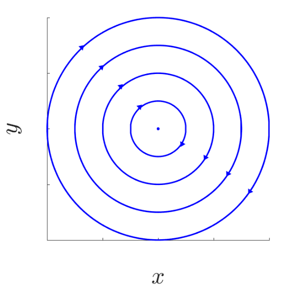
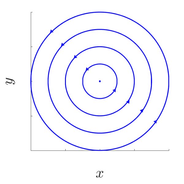
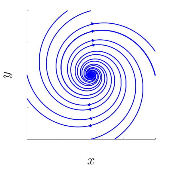
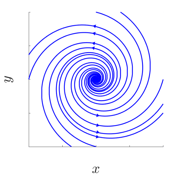
C4. $A$ has $2$ complex eigenvalues $a \pm b$, $b \neq 0$ \(J = \begin{pmatrix}a & -b\\ b & a\end{pmatrix}\)
$A$ not singular:
C1
Trajectory given $O(x_0,y_0) = { (x,y_0(\frac{x}{x_0})^{b/a} \in \mathbb{R}^2: \frac{x}{x_0} > 0)}$
Obtaining the following phase portraits:
| a< b < 0 | a < 0 < b | 0 < a < b |
|---|---|---|
| Stable knot - 2 tangents | Saddle | Unstable knot - 2 tangents |
 |  |  |
C2
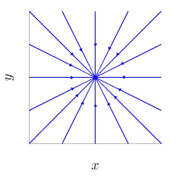
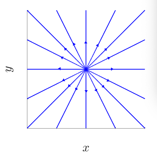
\[\begin{aligned} J &= \begin{pmatrix}a & 0\\ 0 & a\end{pmatrix} \quad a \in \mathbb{R}\backslash \{0\}\\ e^{Jt} &= \begin{pmatrix} e^{at} & 0 \\ 0 & e^{at}\end{pmatrix} \quad \forall\ t \in \mathbb{R}\end{aligned}\]Trajectory given by $O(x_0,y_0) = { (x_0 e^{at}, y_0 e^{at}): t \in \mathbb{R}} = { (x,x\frac{y_0}{x_0}) \in \mathbb{R}^2: \frac{x}{x_0} > 0}$
Obtaining the following phase portraits:
| a < 0 | a > 0 |
|---|---|
| Stable knot - many tangents | Unstable knot - many tangents |
 |  |
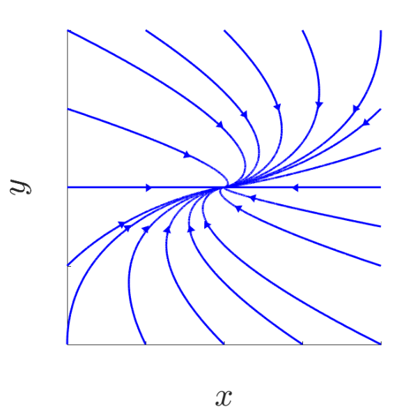
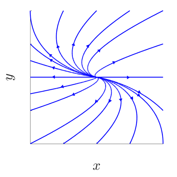
C3
\[\begin{aligned} J &= \begin{pmatrix}a & 1\\ 0 & a\end{pmatrix} \quad a \in \mathbb{R}\backslash \{0\}\\ e^{Jt} &= \begin{pmatrix} e^{at} & te^{at} \\ 0 & e^{at}\end{pmatrix} \quad \forall\ t \in \mathbb{R}\end{aligned}\]Trajectory given by $O(x_0,y_0) = {(x_0 e^{at} + y_0 te^{at}, y_0 e^{at}): t \in \mathbb{R}} = { (\frac{x_0}{y_0}y + \frac{y}{a}\ln \frac{y}{y_0}, y) \in \mathbb{R}^2: \frac{y}{y_0} > 0}$
Obtaining the following phase portraits:
| a < 0 | a > 0 |
|---|---|
| Stable knot - 1 tangent | Unstable knot - 1 tangent |
 |  |
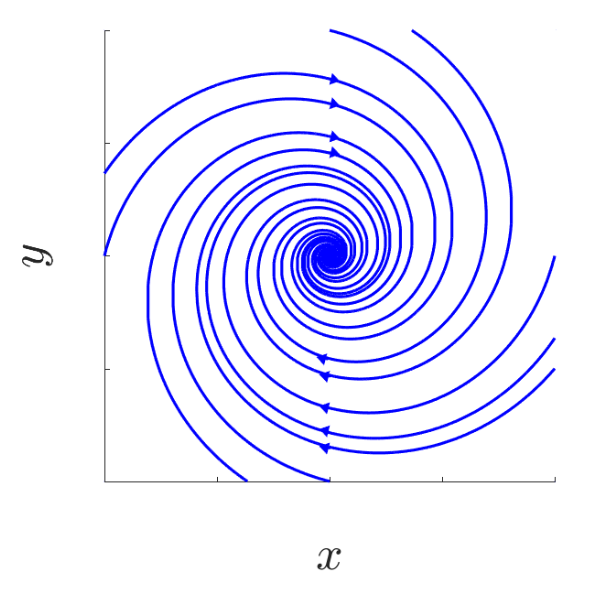
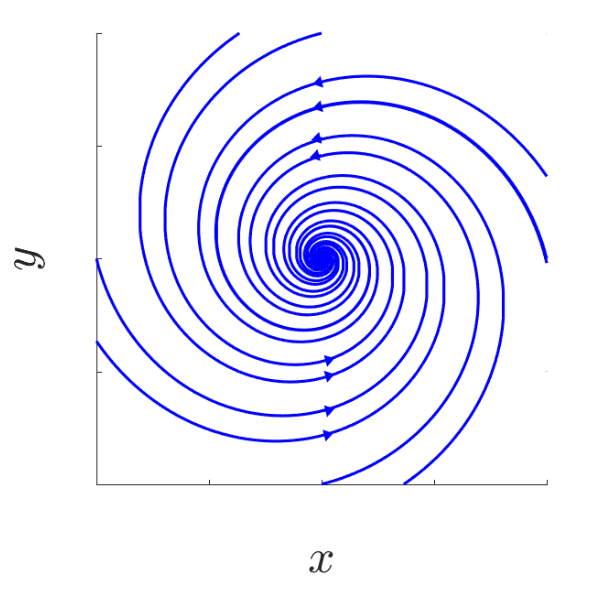
C4
\[\begin{aligned} J &= \begin{pmatrix}a & b\\ -b & a\end{pmatrix} \quad a \in \mathbb{R}\backslash \{0\}\\ e^{Jt} &= e^{at}\begin{pmatrix} \cos (bt) & \sin (bt) \\ -\sin (bt) & \cos (bt)\end{pmatrix} \quad \forall\ t \in \mathbb{R}\end{aligned}\]Trajectory given by $O(x_0,y_0) = { e^{at} \begin{pmatrix} x_0 \cos (bt) + y_0 \sin (bt) \ y_0 \cos (bt) - x_0 \sin (bt) \end{pmatrix}: t \in \mathbb{R}}$
Obtaining the following phase portraits:
| a < 0, b > 0 | a < 0, b < 0 |
|---|---|
| Stable focus | Stable focus |
 |  |
| a = 0, b > 0 | a = 0, b < 0 |
|---|---|
| Centre | Centre |
 |  |
| a > 0, b > 0 | a > 0, b < 0 |
|---|---|
| Unstable focus | Unstable focus |
 |  |
$A$ singular:
C1
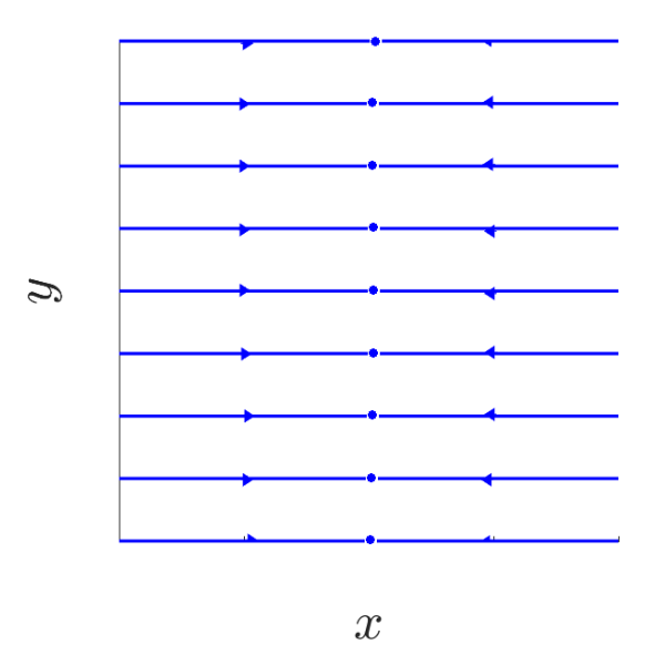
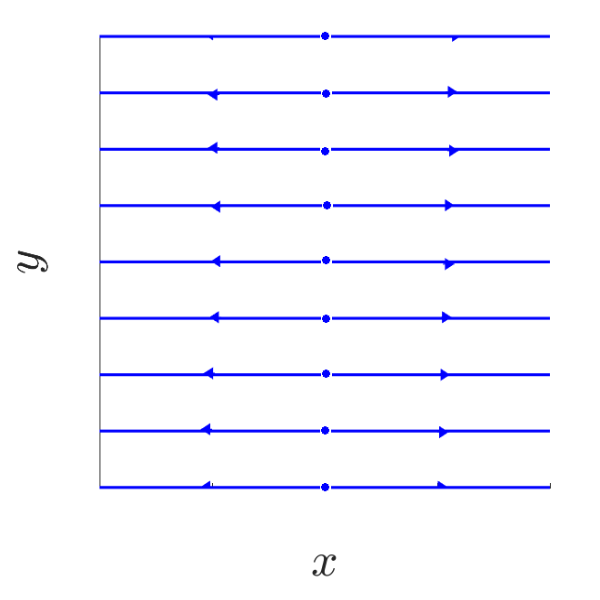
\[\begin{aligned} J &= \begin{pmatrix}a & 0\\ 0 & 0\end{pmatrix} \quad a \in \mathbb{R}\backslash \{0\}\\ e^{Jt} &= \begin{pmatrix} e^{at} & 0 \\ 0 & 1 \end{pmatrix} \quad \forall\ t \in \mathbb{R}\end{aligned}\]Trajectory given by $O(x_0,y_0) = {(e^{at}x_0, y_0) : t \in \mathbb{R}}$
Obtaining the following phase portraits:
| a < 0 | a > 0 |
|---|---|
 |  |
C2
\[J = \begin{pmatrix} 0 & 0\\ 0 & 0 \end{pmatrix}\]Trivially whole space is equilibria
C3
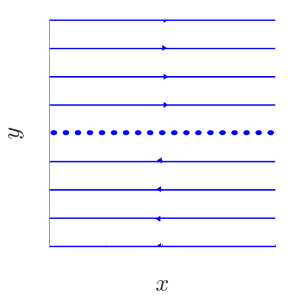
\[\begin{aligned} J &= \begin{pmatrix}0 & 1\\ 0 & 0\end{pmatrix} \quad a \in \mathbb{R}\backslash \{0\}\\ e^{Jt} &= \begin{pmatrix} 1 & t \\ 0 & 1 \end{pmatrix} \quad \forall\ t \in \mathbb{R}\end{aligned}\]Trajectory given by $O(x_0,y_0) = e^{Jt}\begin{pmatrix}x_0 \ y_0 \end{pmatrix}{(x_0 + ty_0, y_0) : t \in \mathbb{R}}$
Obtaining the following phase portraits:
C4
Can’t happen as a 2D matrix of real eigenvalues can’t have eigenvalue of 0.
Remark 3.5 - (Meaning of real + imaginary parts of e.vals of A)
Rate of exponential growth
$Re[e.val]$ - determines rate of exponential growth behaviour of solution \(\lambda(t) = e^{At}\begin{pmatrix}x_0 \\ y_0 \end{pmatrix}\) Obtain exponential growth rate for $\mu (t) = e^{at}$ \(\lim_{t\to\infty}\frac{\ln e^{at}}{t} = a\)Lyapunov exponent
\[\sigma_{lyap}(\lambda) = \lim_{t\to\infty}\frac{\ln \| \lambda (t)\|}{t}\]
For solution $\lambda$ with initial condition $(x_0,y_0) \neq (0,0)$We have a solution decay if $\sigma_{lyap} < 0$ , grow if $\sigma_{lyap} > 0$
Rate of Rotation
Solution rotates is e.vals not real.
For $a+bi$ an e.val$\lvert b \rvert$ - speed of rotation
$sign(b)$ - orientation of rotation
$b> 0 \implies \circlearrowright$
$b< 0 \implies \circlearrowleft$
Jordan Normal Form
Theorem 3.6 - Complex Jordan Normal Form
$A\in \mathbb{R}^{d\times d}, \exists T \in \mathbb{C}^{d\times d}$ s.t we get
With Jordan blocks
\[J_{j}=\left(\begin{array}{ccccc} \rho_{j} & 1 & & 0 & 0 \\ 0 & \rho_{j} & 1 & & 0 \\ & & \ddots & \ddots & \\ 0 & & & \rho_{j} & 1 \\ 0 & 0 & & 0 & \rho_{j} \end{array}\right) \quad \text { for all } j \in\{1, \ldots, p\}\]For $p_j, j \in {1,\dots,p}$ complex e.vals of $A$
Theorem 3.7 - Real Jordan Form
$A \in \mathbb{R}^{d\times d}$, $\exists T \in \mathbb{R}^{d\times d}$ s.t
$J_j$ as in 3.6 if $\rho_j$ real
if $\rho_j$ complex $\implies$
Explicit representation of matrix exponential function
$A \in \mathbb{R}^{d\times d}$
Assume invertible $T \in \mathbb{R}^{d\times d}$ transforms $A$ into real
Proposition 3.8
$A\in \mathbb{R}^{d\times d}$ $J_j, j \in {1,\dots,p}$
Jordan blocks for real Jordan normal form with eigenvalues $\rho_j$
$\rho_j$ real
\[\exp\left\{ \begin{pmatrix}\rho_j & 1 &&0\\ & \ddots&\ddots\\ &&\ddots& 1\\ 0 &&& \rho_j \end{pmatrix}t\right\} = e^{\rho_j t}\begin{pmatrix} 1 & t & t^2/2 & \dots & \frac{t^{d_j -1}}{(d_j -1)!} \\ 0 & 1 & t & \ddots & \vdots\\ && \ddots & \ddots & t^2/2\\ 0 &&& 1 & t\\ 0 & 0 && 0 & 1\end{pmatrix}\]$\rho_j = a_j + ib_j \in \mathbb{C}$
\[\exp\left\{ \begin{pmatrix}C_j & I_2 &&0\\ & \ddots&\ddots\\ &&\ddots& I_2\\ 0 &&&C_j \end{pmatrix}t\right\} = e^{a_jt}\begin{pmatrix} G(t) & tG(t) & \frac{t^2}{2}G(t) & \dots & \frac{t^{d_j -1}}{(d_j -1)!}G(t) \\ 0 & G(t) & tG(t) & \ddots & \vdots\\ && \ddots & \ddots & \frac{t^2}{2}G(t)\\ 0 &&& G(t) & tG(t)\\ 0 & 0 && 0 & G(t)\end{pmatrix}\]Where
\[G(t)=\left(\begin{array}{cc}\cos \left(b_{j} t\right) & \sin \left(b_{j} t\right) \\ -\sin \left(b_{j} t\right) & \cos \left(b_{j} t\right)\end{array}\right)\quad \forall t\ \in \mathbb{R}\]
Exponential growth behaviour
Definition 13. - Spectrum of $A$
\[A\in \mathbb{R}^{d\times d} \quad \Sigma (A) = \left \{ Re(\rho): \rho \text{ eval of } A\right \} = \{s_1,\dots,s_p\}\]For $\dot{x} = Ax$ we have decomposition
\[\mathbb{R}^d = E_1 \oplus \dots \oplus E_q\]$E_j$ invariant
$x\in E_j \implies \varphi(t,x) \in E_j \ \forall t \in \mathbb{R}$
$x \in E_j \backslash {0} \implies \sigma_{lyap}(\varphi(\cdot,x)) = \lim_{t\to\infty}\frac{|\varphi(t,x)|}{t} = s_j$
Definition 14. - semi-simple eigenvalue
If all Jordan blocks associated to eval in real Jordan normal form are:
- 1 dim. for real e.val
- 2 dim. for non-real e.val
Proposition 3.9 - (Exponential estimate for matrix exponential function)
$A\in \mathbb{R}^{d\times d}$, Choose $\gamma > \max \Sigma(A)$
If all e.vals $\rho$ with $Re(\rho) = \max \Sigma(A)$, semi-simple $\implies$ take $\gamma = \max \Sigma(A)$
Variation of constants formula
Proposition 3.10 - (Variation of constants formula)
General solution to $\dot{x} = Ax + g(t)$ given by
Non-linear systems
Stability
Basic definitions
Definition 15.
$x^{\ast}$ an equilibrium of $\dot{x} = f(x) \implies f(x^{*}) = 0$
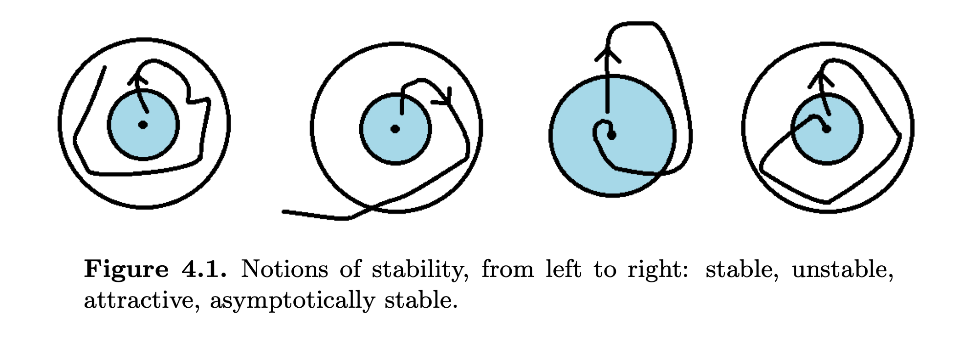
$x^{*}$ stable if $\forall \epsilon > 0, \exists \delta >0$ s.t
\[\|\varphi(t,x) - x^{*}\| < \epsilon \quad \forall x \in B_{\delta}(x^{*}) \text{ and } t \geq 0\]$x^{\ast}$ unstable if not stable
$x^{*}$ attractive if $\exists \delta > 0$ s.t
\[\lim_{t\to \infty}\varphi(t,x) = x^{*} \quad \forall x \in B_{\delta}(x^{*})\]$x^{\ast}$ asymptotically stable if $x^{\ast}$ stable and attractive
$x^{*}$ exponentially stable if $\exists \delta>0, K\geq 1$ and $\gamma <0$ s.t
\[\| \varphi(t,x) -x^{*}\| \leq \| Ke^{\gamma t}\|\]$x^{\ast}$ repulsive if $\exists \delta >0$ s.t $\lim_{t\to -\infty} \varphi(t,x) = x^{\ast}, \forall x \in B_{\delta}(x^{\ast})$
Definition 16. (Homoclinic and heteroclinic orbits)
$\dot{x} = f(x)\ f:\underbrace{D \subset \mathbb{R}^d}_{\text{open}}\to \mathbb{R}^d$ locally Lipschitz continuous, with flow $\varphi$
Orbit $O(x)$ for some $x \in D$
Homoclinic orbit if $\exists$ equilibrium $x^{*} \in D \backslash{x}$ s.t
\[\lim_{t\to\infty}\varphi(t,x) = x^{\ast} \text{ and } \lim_{t\to -\infty}\varphi(t,x) = x^{\ast}\]Heteroclinic orbit if $\exists$ 2 distinct equilibria $x_1^* \neq x_2^*$ s.t
\[\lim_{t\to\infty}\varphi(t,x) = x_1^* \text{ and } \lim_{t\to -\infty}\varphi(t,x) = x_2^*\]
Theorem 7. (Stability of linear systems
Consider autonomous linear system, $\dot{x} = Ax, A \in \mathbb{R}^{d\times d}$
Have trivial equilibrium $x^{\ast} = 0$
- stable $\iff$
- $Re(\rho) \leq 0\ \forall \rho$ e.vals of $A$
- e.val $\rho$ semi-simple $\forall$ e.vals $\rho$ of $A$ with $Re(\rho) =0$
- exponentially stable $\iff Re(\rho) < 0\ \forall$ e.vals $\rho$ of $A$
Hyperbolicity
Definition 17.
$A \in \mathbb{R}^{d\times d}$ hyperbolic if $Re(\lambda) \neq 0\ \forall \lambda$ e.vals of $A$
Equilibrium $x^{\ast}$ of differential equation $\dot{x} = f(x)\ f:D\subset \mathbb{R}^d \to \mathbb{R}^d$ continuouslydifferentiable, is hyperbolic if matrix $f’(x^{\ast}) \in \mathbb{R}^{d\times d}$ hyperbolic.
Lemma 4.9 - Gronwall Lemma
Consider continuous function $u:[a,b] \to \mathbb{R},$ let $c,d \geq 0$
Assume $u$ satisfies implicit inequality
Theorem 8. (Linearised stability)
$\dot{x} = f(x)\ f:\underbrace{D \subset \mathbb{R}^d}_{\text{open}}\to \mathbb{R}^d$ continuously differentiable.
Assume $x^{\ast}$ equilibrium of above s.t $\forall$ e.vals $\lambda \in \mathbb{C}$ of linearisation of $f’(x^{\ast})\in \mathbb{R}^{d\times d}$ we have $Re(\lambda) < 0 \implies x^{\ast}$ is exponentially stable.
Stable and unstable sets, invariant sets
Definition 18. (Stable + unstable set)
$\dot{x} = f(x)\ f:\underbrace{D \subset \mathbb{R}^d}_{\text{open}}\to \mathbb{R}^d$ locally lipschitz continuous, with flow $\varphi$ and equilibria $x^{\ast}$
Stable set of $x^{\ast}$
\[W^{s}(x^{\ast}) = \{ x \in D: \lim_{t\to\infty} \varphi(t,x) = x^{\ast}\}\]Unstable set of $x^{\ast}$
\[W^{u}(x^{\ast}) = \{ x \in D: \lim_{t\to-\infty} \varphi(t,x) = x^{\ast}\}\]Definition 19. (Invariance)
$\dot{x} = f(x)\ f:\underbrace{D \subset \mathbb{R}^d}_{\text{open}}\to \mathbb{R}^d$ locally lipschitz continuous..
positively invariant if $\forall x \in M, O^+(x) \subset M$
negatively invariant if $\forall x \in M, O^-(x) \subset M$
invariant if $\forall x\in M, O(x) \subset M$
Limit Sets
Definition 20. (Omega and alpha limit sets)
$\dot{x} = f(x)\ f:\underbrace{D \subset \mathbb{R}^d}_{\text{open}}\to \mathbb{R}^d$ locally lipschitz continuous, with flow $\varphi, x\in D$
$x_w \in D$ an omega limit point of $x$
\[x_\omega = \lim_{n\to\infty}\varphi(t_n,x)\]
If $\exists$ sequence ${ t_n }{n\in\mathbb{N}}$ s.t $\lim{n\to \infty} t_n = \infty$ and$\omega(x)= {$ all omega limit points of $x}$
$x_{\alpha}\in D$ an alpha limit point of $x$
\[x_{\alpha} = \lim_{n\to\infty}\varphi(t_n,x)\]
if $\exists$ sequence ${t_n}{n\in\mathbb{N}}$ s.t $\lim{n\to\infty}t_n = -\infty$ and$\alpha(x) = {$ all alpha limit points of $x}$
Proposition 4.19 - (Alternative characterisation of limit sets)
$\varphi$ flow of differential from above $x\in D$
Proposition 4.21 - (properties of $\omega,\alpha$ limit sets)
$\dot{x} = f(x)\ f:\underbrace{D \subset \mathbb{R}^d}_{\text{open}}\to \mathbb{R}^d$ locally lipschitz continuous, $x\in D$
$\omega(x)$ invariant
if $O^+(x)$ bounded and $\overline{O^+(x)} \subset D \implies \omega(x) \neq \emptyset$ compact$\alpha(x)$ invariant if $O^{-}(x)$ bounded and $\overline{O^{-}(x)} \subset D \implies \alpha(x) \neq \emptyset$ compact
Lyapunov functions
Definition 21. (Orbital derivatives)
$\dot{x} = f(x)\ f:\underbrace{D \subset \mathbb{R}^d}_{\text{open}}\to \mathbb{R}^d$ locally lipschitz continuous
$V:D\to \mathbb{R}$ continuosly differentiable function.
Define orbital derivative $\dot{V}$ of $V$
$V’(x) \in \mathbb{R}^{1\times d}$ the gradient of $V$ at $x \in D$
$\dot{V}$ describes derivative of $V$ along solution $\mu:I \to D$ of $\dot{x} = f(x)$
Definition 22. (Lyapunov functions)
$\dot{x} = f(x)\ f:\underbrace{D \subset \mathbb{R}^d}_{\text{open}}\to \mathbb{R}^d$ Locally Lipschitz continuous.
$V: D \to \mathbb{R}$ continuously differentiable function
$V$ a Lyapunov function if $\dot{V}(X) \leq 0\ \forall x \in D$
Remark.
Lyapunov function decrease along solutions
Proposition 4.25. - (Sublevel sets of Lyapunov functions are positively invariant)
$\dot{x} = f(x)\ f:\underbrace{D \subset \mathbb{R}^d}_{\text{open}}\to \mathbb{R}^d$
Locally Lipschitz continuous, with Lyapunov function $V:D\to\mathbb{R}$ Any sublevel set of form
\[S_{c} := \{ x\in D: V(x) \leq c\},\ c\in \mathbb{R}\]is positively invariant
Theorem 9. (Lyapunov’s direct method for stability)
$\dot{x} = f(x)\ f:\underbrace{D \subset \mathbb{R}^d}_{\text{open}}\to \mathbb{R}^d$ Locally Lipschitz continuous, $x^{\ast}$ an equilibria and $V:D\to \mathbb{R}$ lyapunov funtion s.t
\[V(x^{\ast}) = 0, V(x) >0 \ \forall x \in D\backslash\{x^{\ast}\} \implies x^{\ast} \text{ stable }\]Theorem 10. (La Salle’s invariance principal)
$\dot{x} = f(x)\ f:\underbrace{D \subset \mathbb{R}^d}_{\text{open}}\to \mathbb{R}^d$ Locally Lipschitz continuous, with Lyapunov function $V:D\to\mathbb{R}$
\[\omega(x) \subset \{ y \in D: \dot{V}(y) = 0\} \ \forall x \in D\]Corollary 4.30 - (Reformation of La Salle’s invariance principle)
$\dot{x} = f(x)\ f:\underbrace{D \subset \mathbb{R}^d}_{\text{open}}\to \mathbb{R}^d$ Locally Lipschitz continuous, with Lyapunov function $V:D\to\mathbb{R}$
Theorem 11. (Lyapunov’s direct method for asymptotic stability)
$\dot{x} = f(x)\ f:\underbrace{D \subset \mathbb{R}^d}_{\text{open}}\to \mathbb{R}^d$ Locally Lipschitz continuous, $x^{\ast} \in D, V:D\to\mathbb{R}$ Lyapunov function s.t
\[\begin{aligned} V(x^{\ast}) =0 &\text{ and } V(x) > 0\ \forall x \in D\backslash\{x^{\ast}\}\\ \dot{V}(x^{\ast}) =0 &\text{ and } \dot{V}(x) < 0\ \forall x \in D\backslash\{x^{\ast}\}\end{aligned}\]$\implies x^{\ast}$ asymptotically stable
Corollary 4.33 - (Sublevel sets of Lyapunov functions are subsets of domain of attraction)
$\dot{x} = f(x)\ f:\underbrace{D \subset \mathbb{R}^d}_{\text{open}}\to \mathbb{R}^d$ Locally Lipschitz continuous, $x^{\ast} \in D, V:D\to\mathbb{R}$ Lyapunov function
Consider sublevel sets of Lyapunov function $V$
$\implies S_c$ subset of domain of attraction $W^{s}(x^{\ast})$ if $S_c \subset D$ compact
Poincaré-Bendixson Theorem
Theorem 12. (Poincare-Bendixson Theorem
$\dot{x} = f(x)\ f:\underbrace{D \subset \mathbb{R}^2}_{\text{open}}\to \mathbb{R}^2$ with flow $\varphi$ continuously differentiable.
Assume for some $x\in D, O^{+}(x) \subset K$ compact $\subset D$
$K$ containing not more than finitely many equilibria.
One of the following 3 hold for $\omega(x)$
$\omega(x)$ a singleton, consisting of an equilibrium
$\omega(x)$ a periodic orbit
$\omega(x)$ consists of equilibria + non-closed orbits
non-closed orbits in $\omega(x)$ converge forward and backward in time to equilibria in $\omega(x)$
$\implies$ either homoclinic or heteroclinic orbits.
Corollary 4.35 - (Existence of a periodic orbit)
$\dot{x} = f(x)\ f:\underbrace{D \subset \mathbb{R}^2}_{\text{open}}\to \mathbb{R}^2$ continuously differentiable with flow $\varphi$.
Assume for $x\in D$, $O^{+}(x) \subset K$ compact $\subset D$
$D$ not containing an equilibrium $\implies \omega(x)$ periodic orbit.